图简介
真实世界的图表
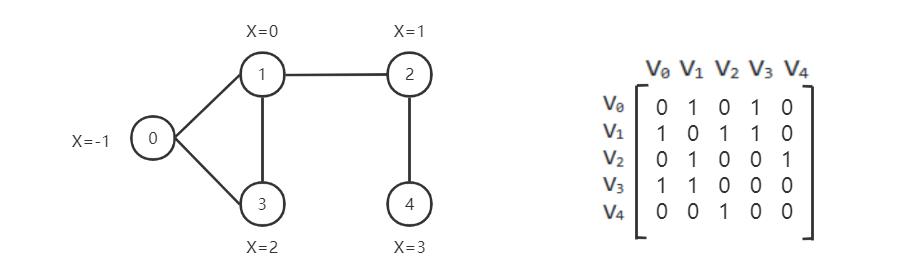
图结构数据已在许多现实世界场景中得到广泛应用。例如,Facebook 上的每个用户都可以被视为一个顶点,而他们之间比如友谊或追随性等关系可以被视为图中的边。 我们可能对预测用户的兴趣或者对网络中的一对节点是否有有连接它们的边感兴趣。
我们可以使用邻接矩阵表示一张图
如何在 CogDL 中表示图形
图用于存储结构化数据的信息,在CogDL中使用cogdl.data.Graph对象来表示一张图。简而言之,一个Graph具有以下属性:
x: 节点特征矩阵,shape[num_nodes, num_features],torch.Tensor
edge_index:COO格式的稀疏矩阵,tuple
edge_weight:边权重shape[num_edges,],torch.Tensor
edge_attr:边属性矩阵shape[num_edges, num_attr]
y: 每个节点的目标标签,单标签情况下shape [num_nodes,],多标签情况下的shape [num_nodes, num_labels]
row_indptr:CSR 稀疏矩阵的行索引指针,torch.Tensor。
col_indices:CSR 稀疏矩阵的列索引,torch.Tensor。
num_nodes:图中的节点数。
num_edges:图中的边数。
以上是基本属性,但不是必需的。你可以用 g = Graph(edge_index=edges) 定义一个图并省略其他属性。此外,Graph不限于这些属性,还支持其他自定义属性, 例如graph.mask = mask。
在Cogdl中表示这张图
|
|
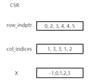
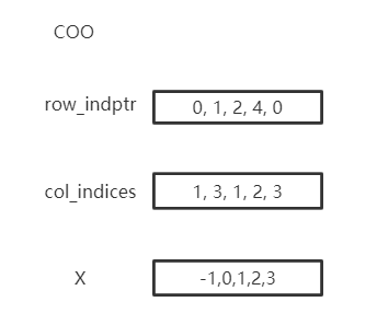
Graph以 COO 或 CSR 格式存储稀疏矩阵。COO 格式更容易添加或删除边,例如 add_self_loops,使用CSR存储是为了用于快速消息传递。 Graph自动在两种格式之间转换,您可以按需使用两种格式而无需担心。您可以创建带有边的图形或将边分配给创建的图形。edge_weight 将自动初始化为1,您可以根据需要对其进行修改。
import torch
from cogdl.data import Graph
edges = torch.tensor([[0,1],[1,3],[2,1],[4,2],[0,3]]).t()
x = torch.tensor([[-1],[0],[1],[2],[3]])
g = Graph(edge_index=edges,x=x) # equivalent to that above
print(g.row_indptr)
>>tensor([0, 2, 3, 4, 4, 5])
print(g.col_indices)
>>tensor([1, 3, 3, 1, 2])
print(g.edge_weight)
>> tensor([1., 1., 1., 1., 1.])
g.num_nodes
>> 5
g.num_edges
>> 5
g.edge_weight = torch.rand(5)
print(g.edge_weight)
>> tensor([0.8399, 0.6341, 0.3028, 0.0602, 0.7190])
我们在Graph中实现了常用的操作:
add_self_loops: 为图中的节点添加自循环
add_remaining_self_loops: 为图中还没有自环的节点添加自环sym_norm:使用 GCN 的 edge_weight 的对称归一化
row_norm: edge_weight 的逐行归一化:
degrees: 获取每个节点的度数。对于有向图,此函数返回每个节点的入度
import torch
from cogdl.data import Graph
edge_index = torch.tensor([[0,1],[1,3],[2,1],[4,2],[0,3]]).t()
g = Graph(edge_index=edge_index)
>> Graph(edge_index=[2, 5])
g.add_remaining_self_loops()
>> Graph(edge_index=[2, 10], edge_weight=[10])
>> print(edge_weight) # tensor([1., 1., ..., 1.])
g.row_norm()
>> print(edge_weight) # tensor([0.3333, ..., 0.50])
subgraph: 得到一个包含给定节点和它们之间的边的子图。edge_subgraph: 得到一个包含给定边和相应节点的子图。sample_adj: 为每个给定节点采样固定数量的邻居
from cogdl.datasets import build_dataset_from_name
g = build_dataset_from_name("cora")[0]
g.num_nodes
>> 2708
g.num_edges
>> 10556
# Get a subgraph contaning nodes [0, .., 99]
sub_g = g.subgraph(torch.arange(100))
>> Graph(x=[100, 1433], edge_index=[2, 18], y=[100])
# Sample 3 neighbors for each nodes in [0, .., 99]
nodes, adj_g = g.sample_adj(torch.arange(100), size=3)
>> Graph(edge_index=[2, 300]) # adj_g
train/eval:在inductive的设置中, 一些节点和边在trainning中看不见的, 对于training/evaluation使用train/eval来切换backend graph. 在transductive设置中,您可以忽略这一点.
# train_step
model.train()
graph.train()

# inference_step
model.eval()
graph.eval()
如何构建mini-batch graphs
在节点分类中,所有操作都在一个图中。但是在像图分类这样的任务中,我们需要用 mini-batch 处理很多图。图分类的数据集包含可以使用索引访问的图,例如data [2]。为了支持小批量训练/推理,CogDL 将一批中的图组合成一个完整的图,其中邻接矩阵形成稀疏块对角矩阵,其他的(节点特征、标签)在节点维度上连接。 这个过程由由cogdl.data.Dataloader来处理。
from cogdl.data import DataLoader
from cogdl.datasets import build_dataset_from_name

dataset = build_dataset_from_name("mutag")
>> MUTAGDataset(188)
dataset[0]
>> Graph(x=[17, 7], y=[1], edge_index=[2, 38])
loader = DataLoader(dataset, batch_size=8)
for batch in loader:
    model(batch)
>> Batch(x=[154, 7], y=[8], batch=[154], edge_index=[2, 338])
batch 是一个附加属性,指示节点所属的各个图。它主要用于做全局池化,或者称为readout来生成graph-level表示。具体来说,batch是一个像这样的张量
以下代码片段显示了如何进行全局池化对每个图中节点的特征进行求和
def batch_sum_pooling(x, batch):
    batch_size = int(torch.max(batch.cpu())) + 1
    res = torch.zeros(batch_size, x.size(1)).to(x.device)
    out = res.scatter_add_(
        dim=0,
        index=batch.unsqueeze(-1).expand_as(x),
        src=x
       )
    return out
如何编辑一个graph?
在某些设置中,可以更改edges.在这种情况下,我们需要在保留原始图的同时生成计算图。CogDL 提供了 graph.local_graph 来设置local scape,任何out-of-place 操作都不会反映到原始图上。但是, in-place操作会影响原始图形。
graph = build_dataset_from_name("cora")[0]
graph.num_edges
>> 10556
with graph.local_graph():
    mask = torch.arange(100)
    row, col = graph.edge_index
    graph.edge_index = (row[mask], col[mask])
    graph.num_edges
    >> 100
graph.num_edges
>> 10556

graph.edge_weight
>> tensor([1.,...,1.])
with graph.local_graph():
    graph.edge_weight += 1
graph.edge_weight
>> tensor([2.,...,2.])
常见的graph数据集
CogDL 为节点分类、图分类等任务提供了一些常用的数据集。您可以方便地访问它们,如下所示:
from cogdl.datasets import build_dataset_from_name
dataset = build_dataset_from_name("cora")

from cogdl.datasets import build_dataset
dataset = build_dataset(args) # if args.dataet = "cora"
对于节点分类的所有数据集,我们使用 train_mask、val_mask、test_mask 来表示节点的训练/验证/测试拆分。
CogDL 现在支持以下的数据集用于不同的任务:
Network Embedding (无监督节点分类): PPI, Blogcatalog, Wikipedia, Youtube, DBLP, Flickr
半监督/无监督节点分类: Cora, Citeseer, Pubmed, Reddit, PPI, PPI-large, Yelp, Flickr, Amazon
异构节点分类: DBLP, ACM, IMDB
链接预测: PPI, Wikipedia, Blogcatalog
多路链接预测: Amazon, YouTube, Twitter
图分类: MUTAG, IMDB-B, IMDB-M, PROTEINS, COLLAB, NCI, NCI109, Reddit-BINARY
Network Embedding(无监督节点分类)
Dataset |
Nodes |
Edges |
Classes |
Degree |
Name in Cogdl |
|---|---|---|---|---|---|
PPI |
3,890 |
76,584 |
50(m) |
— |
ppi-ne |
BlogCatalog |
10,312 |
333,983 |
40(m) |
32 |
blogcatalog |
Wikipedia |
4.777 |
184,812 |
39(m) |
39 |
wikipedia |
Flickr |
80,513 |
5,899,882 |
195(m) |
73 |
flickr-ne |
DBLP |
51,264 |
2,990,443 |
60(m) |
2 |
dblp-ne |
Youtube |
1,138,499 |
2,990,443 |
47(m) |
3 |
youtube-ne |
节点分类
Dataset |
Nodes |
Edges |
Features |
Classes |
Train/Val/Test |
Degree |
Name in cogdl |
|---|---|---|---|---|---|---|---|
Cora |
2,708 |
5,429 |
1,433 |
7(s) |
140 / 500 / 1000 |
2 |
cora |
Citeseer |
3,327 |
4,732 |
3,703 |
6(s) |
120 / 500 / 1000 |
1 |
citeseer |
PubMed |
19,717 |
44,338 |
500 |
3(s) |
60 / 500 / 1999 |
2 |
pubmed |
Chameleon |
2,277 |
36,101 |
2,325 |
5 |
0.48 / 0.32 / 0.20 |
16 |
chameleon |
Cornell |
183 |
298 |
1,703 |
5 |
0.48 / 0.32 / 0.20 |
1.6 |
cornell |
Film |
7,600 |
30,019 |
932 |
5 |
0.48 / 0.32 / 0.20 |
4 |
film |
Squirrel |
5201 |
217,073 |
2,089 |
5 |
0.48 / 0.32 / 0.20 |
41.7 |
squirrel |
Texas |
182 |
325 |
1,703 |
5 |
0.48 / 0.32 / 0.20 |
1.8 |
texas |
Wisconsin |
251 |
515 |
1,703 |
5 |
0.48 / 0.32 / 0.20 |
2 |
Wisconsin |
PPI |
14,755 |
225,270 |
50 |
121(m) |
0.66 / 0.12 / 0.22 |
15 |
ppi |
PPI-large |
56,944 |
818,736 |
50 |
121(m) |
0.79 / 0.11 / 0.10 |
14 |
ppi-large |
232,965 |
11,606,919 |
602 |
41(s) |
0.66 / 0.10 / 0.24 |
50 |
||
Flickr |
89,250 |
899,756 |
500 |
7(s) |
0.50 / 0.25 / 0.25 |
10 |
flickr |
Yelp |
716,847 |
6,977,410 |
300 |
100(m) |
0.75 / 0.10 / 0.15 |
10 |
yelp |
Amazon-SAINT |
1,598,960 |
132,169,734 |
200 |
107(m) |
0.85 / 0.05 / 0.10 |
83 |
amazon-s |
异构图
Dataset |
Nodes |
Edges |
Features |
Classes |
Train/Val/Test |
Degree |
Edge Type |
Name in Cogdl |
|---|---|---|---|---|---|---|---|---|
DBLP |
18,405 |
67,946 |
334 |
4 |
800 / 400 / 2857 |
4 |
4 |
gtn-dblp(han-acm) |
ACM |
8,994 |
25,922 |
1,902 |
3 |
600 / 300 / 2125 |
3 |
4 |
gtn-acm(han-acm) |
IMDB |
12,772 |
37,288 |
1,256 |
3 |
300 / 300 / 2339 |
3 |
4 |
gtn-imdb(han-imdb) |
Amazon-GATNE |
10,166 |
148,863 |
— |
— |
— |
15 |
2 |
amazon |
Youtube-GATNE |
2,000 |
1,310,617 |
— |
— |
— |
655 |
5 |
youtube |
10,000 |
331,899 |
— |
— |
— |
33 |
4 |
知识图谱链接预测
Dataset |
Nodes |
Edges |
Train/Val/Test |
Relations Types |
Degree |
Name in Cogdl |
|---|---|---|---|---|---|---|
FB13 |
75,043 |
345,872 |
316,232 / 5,908 / 23,733 |
12 |
5 |
fb13 |
FB15k |
14,951 |
592,213 |
483,142 / 50,000 / 59,071 |
1345 |
40 |
fb15k |
FB15k-237 |
14,541 |
310,116 |
272,115 / 17,535 / 20,466 |
237 |
21 |
fb15k237 |
WN18 |
40,943 |
151,442 |
141,442 / 5,000 / 5,000 |
18 |
4 |
wn18 |
WN18RR |
86,835 |
93,003 |
86,835 / 3,034 / 3,134 |
11 |
1 |
wn18rr |
图分类
TUdataset from https://www.chrsmrrs.com/graphkerneldatasets
Dataset |
Graphs |
Classes |
Avg. Size |
Name in Cogdl |
|---|---|---|---|---|
MUTAG |
188 |
2 |
17.9 |
mutag |
IMDB-B |
1,000 |
2 |
19.8 |
imdb-b |
IMDB-M |
1,500 |
3 |
13 |
imdb-m |
PROTEINS |
1,113 |
2 |
39.1 |
proteins |
COLLAB |
5,000 |
5 |
508.5 |
collab |
NCI1 |
4,110 |
2 |
29.8 |
nci1 |
NCI109 |
4,127 |
2 |
39.7 |
nci109 |
PTC-MR |
344 |
2 |
14.3 |
ptc-mr |
REDDIT-BINARY |
2,000 |
2 |
429.7 |
reddit-b |
REDDIT-MULTI-5k |
4,999 |
5 |
508.5 |
reddit-multi-5k |
REDDIT-MULTI-12k |
11,929 |
11 |
391.5 |
reddit-multi-12k |
BBBP |
2,039 |
2 |
24 |
bbbp |
BACE |
1,513 |
2 |
34.1 |
bace |